This document contains an overview of how to use the interface in the Mapper package to fully customize the mapper construction. The focus on this document is on package functionality and usage, as opposed the theory the Mapper framework was founded on, and as such discusses Mapper from a strictly algorithmic / computational perspective.
Quickstart
Consider a noisy sampling of points along the perimeter of a circle in \(\mathbb{R}^2\)
set.seed(1234)

## Generate noisy points around the perimeter of a circle
n <- 1500
t <- 2*pi*runif(n)
r <- runif(n, min = 2, max = 2.1)
noisy_circle <- cbind(r*cos(t), r*sin(t))

## Plot the circle
plot(noisy_circle, pch = 20, asp = 1, xlab = "X", ylab = "Y", main = "Circle")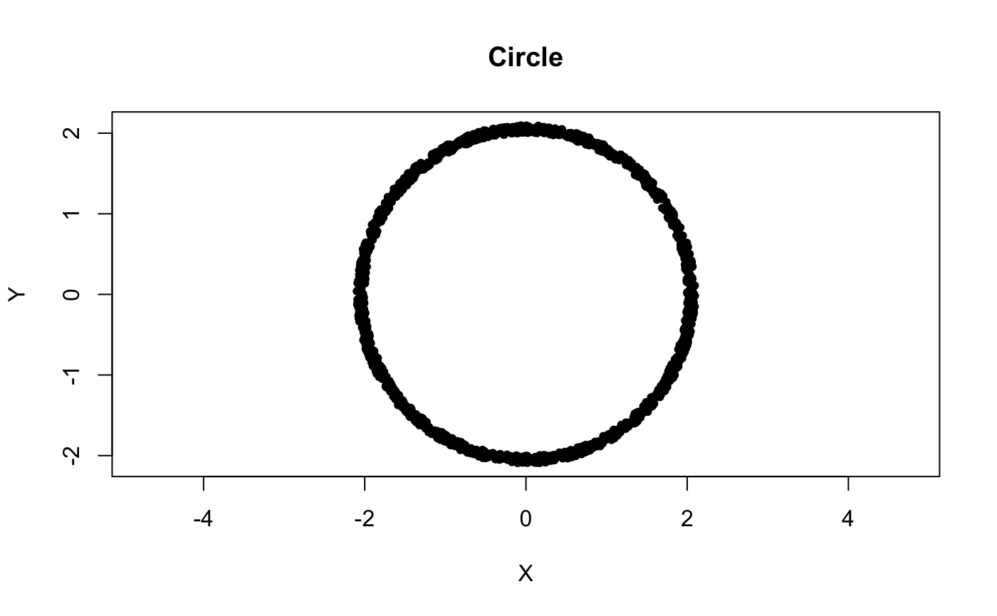
To get the mapper of this circle, first supply the data via X and the mapped values via filter, along with the parameters to other components such as the cover and clustering parameters. See ?mapper for more details. A summary is available with the default print method.
library("Mapper")
left_pt <- noisy_circle[which.min(noisy_circle[, 1]),]
f_x <- matrix(apply(noisy_circle, 1, function(pt) (pt - left_pt)[1]))
m <- mapper(X = noisy_circle,
            filter = f_x,
            cover = list(typename="fixed interval", number_intervals=5L, percent_overlap=50),
            distance_measure = "euclidean",
            clustering_algorithm = list(cl="single"))
print(m)
## Mapper with filter f: X^2 -> Z
## Fixed Interval Cover: (number intervals = [5], percent overlap = [50]%)By default, the core information of the \(1\)-skeleton of the Mapper construction is returned, including:
The vertices, and the points (by index) comprising their corresponding connected components.
Some adjacency representation of the mapper graph
A map between the index set of the cover and the vertices
This is, in essence, all the central information one needs to conduct a more in-depth analysis of the mapper.
Building the Mapper piecewise
For most use-cases, the static method above is sufficient for getting a compact Mapper construction back. However, building the ‘right’ Mapper is usually an exploratory process that requires parameter tuning in the form of e.g. alternative filter functions, ‘fitted’ clustering parameters, different covering geometries, etc. Indeed, the Mapper method itself is sometimes thought of as a tool for exploring properties of the data (as expressed via a filter), whose interconnections reflect some aspects of the metric structure. However, for large data sets, employing this iterative fitting process with the above wrapper method can be prohibitively expensive.
To help facilitate this process, the Mapper package uses R6 class generators to decompose the components used to build the mapper. A few of the benefits R6 classes include full encapsulation support, reference semantics for member fields, easy-to-employ parameter checking via active bindings, and composability via method chaining. More details available at Hadleys Advanced R series or the R6 documentation site.
To demonstrate some of these benefits, consider a simplified interpretation of the Mapper pipeline:
“Filter” the data via a reference map
Equip the filtered space with a cover
Decompose preimages of the (pulled back) open sets of the cover into clusters
Construct the k-skeleton by considering non-empty intersections of the clusters
These steps are demonstrated below using the noisy_circle data set below. To begin building a mapper object more fluidly, one starts by using the MapperRef R6-class instance generator.
The data can be specified at initialization, or later using the use_data method. The format of the data must be either a matrix of coordinate values or a function which returns a matrix of coordinate values.
Assume, as before, that our filter is the distance from every points first coordinate to the point with left-most coordinate, \(p\), i.e.
## 1. Specify a filter function for the data
left_pt <- noisy_circle[which.min(noisy_circle[, 1]),]
f_x <- matrix(apply(noisy_circle, 1, function(pt) (pt - left_pt)[1]))
Coloring the points in the original space w/ a rainbow gradient based on their filter values sheds light on what the filter geometrically represents
## Bin the data onto a sufficiently high-resolution rainbow gradient from blue (low) to red (high)
rbw_pal <- rev(rainbow(100, start = 0, end = 4/6))
binned_idx <- cut(f_x, breaks = 100, labels = F)
plot(noisy_circle, pch = 20, asp = 1, col = rbw_pal[binned_idx], xlab = "X", ylab = "Y", main = "Circle")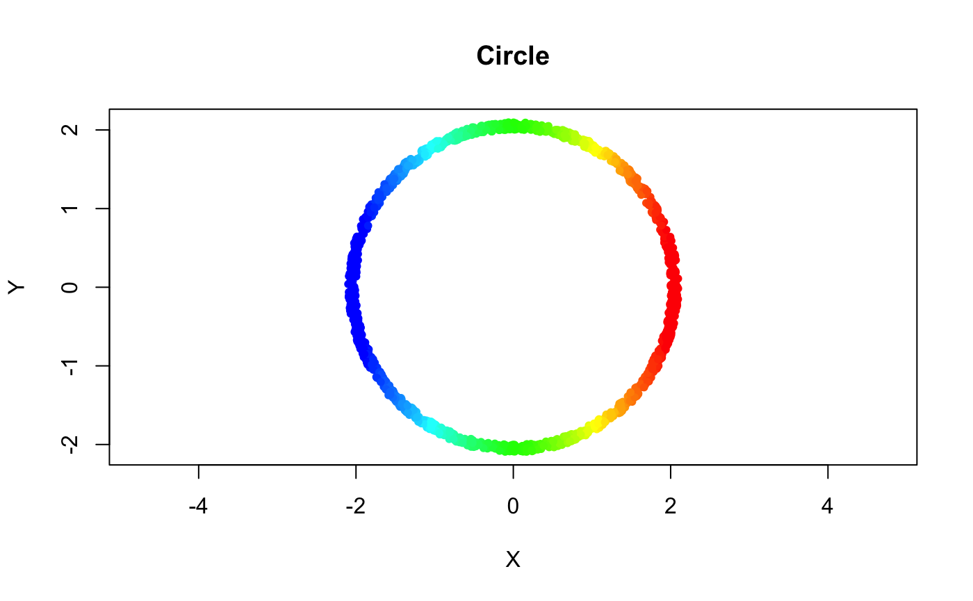
The filter is assigned as usual, and like the data matrix, it accepts a matrix of coordinate values or a function that generates a matrix of coordinate values.
Both the data matrix and filter as stored as functions, which both accept as input a set of indices and return as output a matrix of coordinate values.
Constructing the cover
Once the filter has been applied, a cover must be chosen to discretize the space. Here, a simple rectangular cover with fixed centers is used.
Cover parameters may be be supplied at initialization, or set via the assignment operator. If you supply a single value when the filter dimensionality \(> 1\), the argument is recycled across the dimensions. The cover summary can be printed as follows:
## Fixed Interval Cover: (number intervals = [5], percent overlap = [20]%)Once parameterized, the cover may be explicitly constructed via the construct_cover member, before passing back to the MapperRef instance. The construct_cover function uses the given set of parameters to populate the intersection between the open sets in the cover and the given filter data.
cover$construct_cover(filter = m$filter) ## Now the level sets are populated
summary(cover$level_sets)
## Length Class Mode
## (1) 459 -none- numeric
## (2) 269 -none- numeric
## (3) 234 -none- numeric
## (4) 258 -none- numeric
## (5) 456 -none- numericMapper accepts any cover that derives from the abstract CoverRef R6 class. Any such derived cover instance can be assigned to the $cover member.
A few covering methods often used in practice are available. To see a list, use the covers_available method.
## Typename:                    Generator:                         Parameters:
##  fixed interval               FixedIntervalCover                 number_intervals, percent_overlap
##  restrained interval          RestrainedIntervalCover            number_intervals, percent_overlap
##  ball                         BallCover                          epsilon
If you want to use a cover outside of the ones offers by the package, feel free to derive a new type cover class (and submitting a pull request!). There’s also a small tutorial on how one might go about making their own.
Decomposing the preimages
After creating the cover, the next step is to perform the pullback operation, wherein the cover \(\mathcal{U}\) of the space \(Z\) is used to create a cover on \(X\) through \(f\). This operation generally denotes two operations: computing the preimages of each open set, and decomposing the subsets of \(X\) given by these preimages into connected components. The latter is referred to in the original Mapper paper as partial clustering, and it (naturally) requires a number of parameters.
The goal of the Mapper package is to provide the user full access to how the open sets are decomposed, while also providing easy-to-parameterize defaults for those unfamiliar with clustering in general. Towards this end, there are two options to assign the clustering algorithm: either choose from a set of pre-defined clustering algorithms (+ hyper-parameters), or simply supply your own function to do the decomposition.
Using pre-configured defaults
For people do not have much experience in clustering, one may simply one of many pre-defined linkage criteria to the cl argument of the use_clustering_algorithm method. The choice of linkage criteria determines the type of hierarchical clustering to perform. Given a cluster hierarchy, it’s common to cut the tree at some height value to obtain a partitioning of the points. There are a few available cutting heuristics implemented which attempt to identify the major ‘clusters’ automatically. See ?use_clustering_algorithm for more details.
Below is an example of how to specify a pre-configured clustering approach.
For a complete list of the available linkage criteria, see ?stats::hclust.
Using a custom function
If it is not sufficient to use one of the standard clustering methods, you can alteratively just supply your own clustering function. The only requirement is that it take input the index of the open set pid, a vector of indices idx\(\subset \{1, 2, \dots, n\}\) (representing the preimage), and the mapperRef instance object self, and return an integer vector giving a partitioning on that subset. An example of how one might construct a custom clustering function leveraging the parallelDist and fastcluster packages is given below.
custom_clustering_f <- function(num_bins.default = 10L){
  dependencies_met <- sapply(c("parallelDist", "fastcluster"), requireNamespace)
  stopifnot(all(dependencies_met))
  function(pid, idx, self) {
    dist_x <- parallelDist::parallelDist(self$X(idx), method = self$measure)
    hcl <- fastcluster::hclust(dist_x, method = "single")
    eps <- cutoff_first_bin(hcl, num_bins = num_bins.default)
    cutree(hcl, h = eps)
  }
}
m$use_clustering_algorithm(cl = custom_clustering_f(10L))
The above example also demonstrates a simplified example of what one of the pre-configured options might look like. Functions supplied via the use_clustering_algorithm accessor are given access to the instance fields and methods, e.g. the data self$X(...) and the measure with self$measure.
By default, the metric to cluster on is set to euclidean distance. However, the distance measure may also be any one of the 49 (at this time of writing) proximity measures available in from the proxy package. To change the distance measure, use the use_distance_measure method.
For a complete list of the distance/similarity measures supported, see ?proxy::pr_DB.
Notice the clustering function in this example was created as a closure. Since closures capture their enclosing environments, they can be quite useful for e.g. storing auxiliary parameters, validating package dependencies (e.g. as above), caching information for improved efficiency, etc. However, for the same reason, they are a common cause of a form of memory leaking if used carelessly, so they should be used with mindfully.
Performing the decomposition
Once the clustering algorithm has been picked the pullback, also called the inverse image, can be constructed.
In the Mapper package, $construct_pullback applies the clustering algorithm to the preimages of given cover, populating the vertices the mapper construct. A mapping between the index set and the vertex labels is also recorded.
##   0   1   2   3   4   5   6   7
## 459 133 136 129 105 132 126 456## List of 5
## $ (1): num 0
## $ (2): num [1:2] 1 2
## $ (3): num [1:2] 3 4
## $ (4): num [1:2] 5 6
## $ (5): num 7Constructing the k-skeleton
The final step to create a Mapper is to construct the geometric realization of the pullback cover: a simplicial complex. Internally, the simplicial complex Mapper computes is stored in a Simplex Tree. The underlying simplex tree is exported as an Rcpp Module, and is accessible via the $simplicial_complex member.
## < empty simplex tree >The simplex tree is a type of trie specialized specifically for storing and running general algorithms on simplicial complexes. For more details on the simplex tree, see use ?simplextree, or see the package repository, and references therein.
The construction of the simplicial complex is achieved by creating a \(k\)-simplex for each non-empty \((k + 1)\)-fold intersection. Often, instead of constructing the full-dimensional complex (where the dimension is governed by the maximum number of non-empty intersections in the cover), it’s common to restrict the mapper to the k-skeleton of the nerve instead.
With the Mapper package, each dimension can be specified (and parameterized) independently, i.e.
## Simplex Tree with (8, 8) (0, 1)-simplicesThe reason for this design is that, for some practical applications, there may be dimension-dependent operations one may want to isolate. For example, if instead of modifying the complex directly, you want to just get the \(k\)-simplices that would be added to complex, i.e. had a non-empty intersection, you can specify modify=FALSE
##      [,1] [,2]
## [1,]    0    1
## [2,]    0    2
## [3,]    1    4
## [4,]    2    3
## [5,]    3    6
## [6,]    4    5
## [7,]    5    7
## [8,]    6    7
Just like the $construct_pullback method, $construct_nerve optionally accepts a subset of indices which can be used to restrict the intersection computation to specific subsets of the data. For example, the following only considers non-empty intersections between vertices whose connected components intersected the sets indexed by “(1)” and “(2)”
## This checks the pairs given by: expand.grid(v1=m$pullback$`(1)`, v2=m$pullback$`(2)`)
m$construct_nerve(k = 1L, indices = matrix(c("(1)", "(2)"), nrow = 1))
In this way, the $construct_nerve method allows one to obtain finer control over how exactly either individual pairs of subsets or individual dimension of the simplicial complex are constructed. If one just wants to construct \(k\)-simplices for all non-empty intersections up to some dimension of \(k\), e.g. to reduce the mapper to its graph representation, the \(1\)-skeleton may be computed as follows.
## Simplex Tree with (8, 8) (0, 1)-simplicesEach call to construct_k_skeleton clears out the simplicial complex, decomposes the preimages into vertices, and then iteratively builds the nerve up to the specified dimension. Constructing the skeleton this way is an idempotent operation: it can safely be called redundantly, and should always return the same result (assuming the clustering algorithm is deterministic).
Putting it all together
The above is a brief exposition into the various components of the MapperRef object. Generally speaking, obtaining an ‘accurate’ mapper representation of data may require careful tweaking. This package attempts to enable the configurability one might need to obtain that representation.
To streamline this process, the Mapper packages relies on method chaining to allow composability. That is, by convention, all the methods denoted with the use_* enact side-effects on the MapperRef object and return the instance invisibly. This enables a reduction of the Mapper pipeline to a sequence of chained operations:
m <- MapperRef$new()$
  use_data(noisy_circle)$
  use_filter(filter = f_x)$
  use_cover(cover = "fixed interval", number_intervals = 5L, percent_overlap = 20)$
  use_distance_measure(measure = "euclidean")$
  use_clustering_algorithm(cl = "single")$
  construct_pullback()$
  construct_nerve(k = 0L)$
  construct_nerve(k = 1L)
Practical defaults and wrappers are available to simplify this even further. In particular, the default distance measure is euclidean, the default clustering algorithm is single-linkage w/ a sensible cutting heuristic, etc. Thus, the above can also be constructed with:
m <- MapperRef$new(noisy_circle)$
  use_filter(filter = f_x)$
  use_cover(number_intervals = 5L, percent_overlap = 20)$
  construct_k_skeleton(k = 1L)
If the Mapper is constantly being reparameterized, this interface is preferred over the more concise mapper call because of the efficiency that comes with mutability. To illustrate this, consider the case where you want to use a different distance measure for the clustering algorithm. To change the metric with the ‘static’ approach, one might do something like the following:
all_params <- list(
  X = noisy_circle,
  filter = f_x,
  cover = list(cover="fixed interval", number_intervals=10L, percent_overlap=50),
  clustering_algorithm = list(cl="single", cutoff_method="histogram", num_bins=10L)
)

m_static1 <- do.call(mapper, append(all_params, list( distance_measure = "euclidean")))
m_static2 <- do.call(mapper, append(all_params, list( distance_measure = "mahalanobis")))
Both function calls require the entire mapper to be reconstructed, including the cover, the allocation for the simplex tree, all initializers, etc. With reference semantics, you can keep all the same settings and just change what is needed. For example, the following switches the distance measure and exports mapper objects without reconstructing the cover:
m_dynamic <- lapply(c("euclidean", "mahalanobis"), function(measure){
  m$use_distance_measure(measure)$
    construct_k_skeleton(k=1L)$
    exportMapper()
})
Note that, due to the a natural dependency chain that comes with Mapper, the pullback and nerve operations both needed to be recomputed (via construct_k_skeleton), since the latter depends on the former, and the former depends on the distance measure. Determining what requires recomputing depends on how far up the dependency chain you go. For example, consider recomputing the 1-simplices with different intersection size thresholds.
invisible(lapply(1:10, function(e_weight){
  m$construct_nerve(k = 1L, min_weight = e_weight)
  # ... $exportMapper()
}))
In this case, compared to the static method, we save on needing to recompute the cover, the clustering, and the construction of the pullback.
Visualizing the Mapper
The pixiplex package provides a htmlwidget implementation of a subset of the pixi.js geared for visualizing and interacting with simplicial complexes, which can be used to visualize the mapper construction. An export option is available via the $as_pixiplex function, which provides a few default coloring and sizing options.
For more information, see the package repository.
For a static rendering of the mapper, one can use either the as_igraph method or, for higher-order complexes, the default S3 plot method available in the simplextree package (e.g. plot(m$simplicial_complex)). Other options for visualization are an ongoing effort. If you have a particular visualization package you prefer, feel free to submit a issue or PR on the github repository.